Fundamentals of Sound MODULE 2A: BASIC ACOUSTICS Vibrations - Signals - Spectra - Envelopes - Waves

Physical attributes of acoustic waves - Part I: Introduction

For an alternative self-study resource see Sound Waves (University of Salford)
 

   

Oscillation: A broad term, describing the variation (back-and-forth) of any physical or other property of a system around a reference value. The reference value is not fixed for each system. Rather, it is always defined (and re-defined) in the context of some question of interest. To appreciate this generalization consider the following example: Relative to the earth's center (i.e. with the earth's center as the reference point and simplifying the earth as a sphere), a given point on the earth's surface moves in a circle. Relative to the sun's center, the same point moves in a circular spiral. Relative to the center of our galaxy, the same point moves in a helical spiral, ... and so on. See to the right.
Vibration: A mechanical phenomenon, special case of oscillation: the back-and-forth motion of a mass around a point of reference, called point of rest or equilibrium. More Generally:   Equilibrium: the condition arising when all forces applied to a system are perfectly balanced. Unstable equilibrium: equilibrium that breaks down if disturbed (first image, below).    Stable equilibrium: equilibrium that is maintained in spite of disturbances (second image, below).  All musical instruments (and, more generally, all vibrating objects) operate under stable equilibrium conditions. During equilibrium there is no vibration and no potential for sound. When performers pluck a guitar string, blow into a trumpet, or strike a drum, they apply a force that disturbs the given equilibrium, initiating vibrations that can produce sound. Some time after they stop applying any force, the vibrations stop and the string / air column / drum head returns to its equilibrium state, due to friction "consuming" the energy that initiated the vibration. Vibrations vs Waves: In most cases, observations on the vibrations of a sound source have corresponding features in the resulting sound waves, and observations on sound waves have more-or-less direct origins in vibrations.  Exceptions to such correspondence are rare but important and were first identified by Lord Rayleigh (John W. Strutt) in the late 1800s. We'll discuss some of them in the second half of the module.
Simple Harmonic Motion: the simplest type of vibration; for example, a free pendular motion. See the animation to the right (top). In a simple harmonic motion, the restoring force, F=m*a (i.e. force pulling the vibrating mass m back towards its point of rest at an acceleration (a)) is proportional to the displacement (distance away) from its resting point.   Simple harmonic motion can be described graphically by a sinusoidal curve, usually referred to as  sine curve / sine signal. Such curves/signals are described by the following equation:   y(t) = Asin(2πft+φ). For our course, you only need to develop a qualitative understanding of this equation.   In a signal that represents a simple harmonic motion y: displacement (y axis)     t: time (x axis)    A: amplitude or maximum displacement - for sine signals this is constant, represented by a single point on the y axis,     f: frequency (cycles/s) φ (or θ): starting phase/angle in the cycle (1 cycle=2π=3600    π: 3.14...)   The animation to the right (bottom), illustrates the relationship between steady circular motion and sinusoidal motion.
Optional: The video, below, explains in detail what the sinusoidal equation means and how it has been derived (from Khan Academy's high-school AP physics resources).

 

Complex vibration/wave:  a vibration in which the restoring force is related to displacement in a complex way. Complex vibrations are described graphically by complex curves. All such vibrations can be seen as the result of the combination of multiple simple harmonic motions. By extension, the curves/signals that describe them are essentially the sum of an appropriate number of sine curves/signals. We will return to this when we discuss "Spectrum". Practically all sounds we encounter or create correspond to complex waves, which have their origin in complex vibrations and are represented by complex signals, which, in turn, can be derived from (analyzed into) some set of sine signals.

 

(Acoustical) Signal:  A two-dimensional graphic representation of a vibration/wave, plotting displacement (distance from the point of rest), or a number of other level-related variables such as velocity, pressure, etc. (y or vertical axis), over time (x or horizontal axis). A signal is therefore a "time-domain representation" showing how some variable changes with time. Signals of waves are also referred to as waveforms. Sinusoidal/Sine signals represent sinusoidal vibrations/waves and complex signals represent complex vibrations/waves.
The signal, above, with its regular, sinusoidal peaks and valleys, represents a simple/sine/pure wave, corresponding in frequency to the note A3. The peaks of the signal appear at regular intervals of 4.54 milliseconds, or 0.00454 seconds, or 1/220th of a second. So the Period of the signal is 1/220th of a second. This means that the signal (and the wave it represents) repeats itself 220 times per second or has a Frequency of 220 Hertz (Hz).	The signal, above, also represents a sine wave. This one corresponding in frequency to the note A4. This signal repeats twice as fast as the one to the left, at a frequency of 440 Hz. The vibration it represents would travel through air to our ear about as quickly as the one represented to the left, but would cause the air molecules to vibrate at a rate twice as fast.
The Amplitude of both signals is represented by the distance between the top (or bottom) peak and the central horizontal line, representing the point of rest (equilibrium).
	The Signal Envelope is a boundary curve that traces the signal's amplitude through time and, consequently, captures how energy in the signal changes with time. It encloses the area outlined by all maxima of the motion represented by the two-dimensional signal and includes points that do not belong to the signal (in the images: signal is in blue, envelope is in red).    For sinusoidal signals, the envelope is a horizontal straight line, parallel to the x axis (see above). For all other signals, the envelope has a different shape, made out of separate time stages/portions.   The terms describing a signal envelope's stages can be confusing. We will adopt the terminology illustrated below left, used in digital filter and synthesizer design. The image below right (signal of a trombone tone) illustrates the more common envelope stage terminology, employed by musicians.   Signal envelopes and spectral envelopes (will be described under "Spectrum") are the two features that audio engineers are most likely to manipulate. We will be devoting substantial time to the exploration of their physical and perceptual correlates.
The attack stage captures how energy rises in a signal from 0 to its maximum level. Its signal shape and corresponding sonic characteristics depend on the inertia characteristics of the sound source (related to source material, shape, tension, etc.) and to the type of excitation (i.e. plucked, bowed, blown, struck, etc.). It is perceptually salient (i.e. noticeable/characteristic), particularly so for impulse signals where the attack portion contains most of the signal's energy.  The decay portion captures how vibration energy in a system settles, following initial excitation and assuming continuous excitation. For physical/natural (as opposed to electronic or digital) sound sources, the decay stage is the shortest envelope stage. The sustain stage captures how a sound source responds during continuous excitation. It is the most regular/periodic of the envelope stages and, for continuous signals, contains a sound's most salient features. (Note: in acoustics, "sustain" is frequently called "steady state," even though neither it's amplitude nor its spectral envelopes remain truly steady with time). The release stage captures how energy in a system naturally dies out following the end of energy supply. In most cases, the release stage is longer than the attack stage with the natural resonant frequencies of a sound source dying out last. The broader the resonant response of a source the richer and shorter the release stage (more during the next module, under "Resonance"). Impulse signals: signals resulting from the instantaneous (very short) excitation of a sound source, which is then left to vibrate on its own until the energy dies out (due to some form of friction/resistance). Impulse signals only include the attack and release (decay) envelope portions.   Continuous signals: signals resulting from continuous excitation of a sound source. Continuous signals include all four signal envelope portions, occurring in this order: attack, decay, sustain, release.

  
 

Periodic vibration/wave: A vibration/wave that repeats itself at regular time intervals. Periodicity and regularity are attributes with specific perceptual significance. In general, regularity encourages prediction. In terms of sound, periodic waves give rise to well-defined pitch sensations.   Period (T): The time it takes to complete a single full vibration/wave cycle, represented on the x axis of a signal. Period is measured in seconds/cycle and is the inverse of frequency f.  T=1/f . Note that time (t) and period (T) are related concepts but do not describe the same thing, which is why they are represented by different symbols.
Frequency (f): Number of repetitions per unit time. Number of cycles per second. It is measured in Hertz (Hz): 1 Hz = 1 cycle/second. Frequency values are not directly represented by signals. They are represented indirectly by period values T=1/f, measured in seconds per cycle on the x axis. So, f=1/T. Frequency values are directly represented on the x axis of a spectrum (see the section on "Spectrum," further below). The relationship between rotation at a steady angular velocity (i.e. steady rotation at fixed values in angle-degrees/s) and vibration at a steady frequency (i.e. sinusoidal motion at fixed values in cycles/s) has been illustrated under "simple harmonic motion," above. Changes in frequency correspond primarily to changes in pitch.
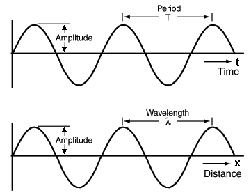
Amplitude (A): Maximum displacement (velocity, pressure, etc.) away from the point of rest. For sine signals, amplitude is represented as a single point on the y axis. Note: for sound waves, displacement amplitudes of air molecules are minute (~ 1 millionth of an inch for speech). As already noted, the y axis represents displacement (move away) from equilibrium (point of rest) as time passes, which has different values at different moments in time. For a given sine signal, the maximum such value is that signal's amplitude. For complex signals, amplitude is represented by a subset of points on the y axis of , tracked by the signal envelope. For spectra, amplitude is represented by the entire y axis, which describes the total energy per frequency or frequency band within a signal (more in the section on "Spectrum," further below). Changes in amplitude correspond primarily to changes in loudness.

 

Phase: Position on the vibration cycle at a given moment in time. Changes in the absolute phase values of non-simultaneous signals are not perceptible. e.g. If the signals, below, were played in succession they would sound identical, in spite of the fact there is a phase-shift (time-lag) among them. The same is the case for signals played simultaneously but having very different frequencies. So, changes in the phase relationship among the spectral components of any given harmonic complex signal (see "Spectra", below) have no perceptual effect (examples).

In contrast, changes in phase relationships among multiple simultaneous signals, that are identical or close in frequency, are quite salient and correspond to loudness, timbre, pitch, and perceived source-location changes, to be described later in the course (click on the image, below, for an example of phase-shift's influence on timbre).

  
 

 

Logarithmic Scale for Power, Intensity, and Pressure

 

Intensity (I): A measure of the amount of energy a vibration (wave) produces (carries) per second, through a unit area. Defined as Power over Area. Measured in Watts per square meter (W/m²).
Power is proportional to the square of amplitude (A²) to the square of frequency (f ²) and, for waves in gases & liquids, to the square of pressure (P²).
The key takeaway message from this relationship is that producing higher amplitudes/frequencies requires (emits) exponentially higher amounts of energy.

The absolute units for Power (Watts), Intensity (Watts/m²), and Pressure (Pacals or N/m²) are all linear. However, when applied to sound, all these quantities are usually expressed on a 10-base logarithmic (log) scale.

 

---

Short review of logarithms and logarithmic operations
 
Logarithms are complimentary to powers.

Reminders: 10³ = 10x10x10 = 1000;     2⁴ = 2x2x2x2 = 16;      3² = 3x3 = 9
 
                     10⁵ x 10³ = 10⁵⁺³ = 10⁸
                     10⁵ / 10³ = 10^5-3 = 10²
                     10³ / 10⁵ = 10^3-5 = 10^-2 = 1/10²

Logarithm - General Definition: The log with base x of a number y is the power a to which we must raise the base, x, in order to get y.

So, when we say that the x-base log of a number y is equal to a we mean that, in order to get y we must raise x to the power of a:
In math notation: log_xy = a  <=>  y = x^a .  [by definition, log_x1 = 0].
For example:
   log₁₀10 = 1  because 10 = 10¹
   log₁₀1000 = 3  because 1000 = 10³
   log₁₀2 = 0.3  because 2 = 10^0.3
   log₂2 = 1  because 2 = 2¹
   log₂8 = 3  because 8 = 2³
   log₂10 = 3.322  because 10 = 2^3.322
 

Addition in log math is equivalent to multiplication in linear math.
For example:
    log₁₀1000 + log₁₀100 = log₁₀10³ + log₁₀10² = 3 + 2 = 5 = log₁₀10⁵ = log₁₀100,000 = log₁₀(1000 * 100)
 
Similarly, subtraction in log math is equivalent to division in linear math.
For example:
    log₁₀1000 - log₁₀100 = log₁₀10³ -  log₁₀10² = 3 - 2 = 1 = log₁₀10¹ = log₁₀10 = log₁₀(1000/100)

---

 

There are two reasons why we use log rather than linear scales to measure sound Power, Intensity, and Pressure:
 
a) As stated in Fechner's Psychophysical Law (mid 1800s), perception relates (approximately) logarithmically to physical stimuli: multiplication in the value of a physical stimulus corresponds to addition in the resulting sensation. 
Therefore, log math provide a better model to the relationship between physics (waves) and sensation (sound) than linear math.
 
b) Log math permit the compression of very large scales into smaller and easier manageable ranges, which are still fine enough to match the resolution of perception. For example, the linear range between the smallest (barely perceptible at 1,000Hz) and largest (harmful to the ear) audible Intensities is |10^-12 to 1 W/m²|,  amounting to 1,000,000,000,000 steps.
In contrast the same range in log math is |log₁₀10^-12 - log₁₀1| = |-12-0| = 12 Bells (after A.G. Bell) or 120 decibels (dB) ("deci-": Latin for "one tenth").

Smallest perceivable, or REFERENCE sound level: 0dB (less than 1 billionth of change in atmospheric pressure)
0dB corresponds to a) Power = W_ref = 10^-12 W,  b) Intensity = I_ref = 10^-12 W/m², and  c) Pressure = P_ref = 2*10^-5 Pa (N/m²)
Largest safe sound level: 120dB
120dB corresponding to a) Power = 1 W,   b) Intensity = 1 W/m², and   c) Pressure = 20 Pa (N/m²)
 
Sound level measurements assume 10-base log values and the base is usually omitted form the notation. So: log₁₀10^-12 = log10^-12

We are ultimately interested in the sensation of sound rather than simply in physical waves. So, we express Power, Intensity, and Pressure levels of a sound logarithmically, in dB (i.e. 1/10 of a Bell), essentially comparing absolute power/intensity/pressure values to the corresponding reference values.
Sound Power Level: SWL =  10* log W/W_ref 
Sound Intensity Level: SIL = 10*log I/I_ref 
Sound Pressure Level: SPL = 20*log P/P_ref  (Optional: why the constant for SPL is 20  but for SWL and SIL is 10?)

The main takeaway messages from discussing these equations are:
a) log sound levels in dB are not absolute but relative to some reference level corresponding to "barely audible";
b) dB levels derive from ratios of physical quantities and are therefore unit-less;
c) one cannot perform math operations (addition/subtraction/multiplication/division) on dB the same way one would do with linear (regular) numbers.

Key logarithmic facts to memorize about sound level and frequency (bookmark this online dB calculator for future use):

Sound Level facts (more in the "Loudness" module)

• Doubling (halving) the sound level corresponds to +3dB (-3dB).
  e.g. a) two guitars at 65dB each combine to produce 68dB;
         b) cutting in half the number of instruments in an orchestra that produces 85dB, will result in an orchestra that produces 82dB.
   

• 10-fold Increase (decrease) in sound level corresponds to +10dB (-10dB) and to "twice (half) as loud";
  100-fold Increase (decrease) in sound level corresponds to +20dB (-20dB);
  1000-fold increase (decrease) in sound level corresponds to +30dB (-30dB), and so on.
  e.g. a) to increase an orchestra's average level by 20dB you need to combine it with another 99 identical orchestras;
          b) reducing the sound entering/escaping a recording studio by 30dB corresponds to blocking 99.9% of the original sound energy.

Frequency facts (more in the "Pitch" module)

• Successive doublings of a frequency produce tones that sound progressively higher in pitch but, at some level, also identical and perfectly blending when heard simultaneously (e.g. all notes with the same letter name / 1 or more octaves apart).
   

• Integer multiples of a frequency produce tones that blend into a single tone perception when heard simultaneously.

See also an additional table of commonly encountered sound levels.
We will return to this topic during our discussion on loudness.

Root-Mean-Square (Pressure) Amplitude

The amount of energy in a signal can be measured in terms of a) 0-to-peak amplitude (maximum positive displacement away from rest; standard amplitude measure in the equation for the simple harmonic motion and in sinusoidal signals), b) peak-to-peak amplitude (difference between positive and negative maximum displacement away from rest; useful when describing energy content of signals that are not symmetrical around the time axis; e.g. most signals generated by musical instruments) c) root-mean-square (RMS) amplitude (for sinusoidal signals, RMSAmplitude = 0.707*PeakAmplitude).  For example, root mean square Pressure or PRMS is a measure of the area outlined by the signal (see Figure b, below) and is defined as the square root of the average of the square of the pressure of the sound signal over a given duration (usually one period): PRMS = (P2)average0.5  To calculate the RMS of any set of numbers:      i) square each number in the set,      ii) calculate the set's average and      iii) calculate the square root of the average. This is the only way to calculate a valid average (mean) value for quantities that, like sound signals, oscillate between positive and negative values. For example, just calculating the straight average amplitude over one or more full cycles would result in 0 for all sine signals.

For sine signals, peak and RMS amplitudes are interchangeable since their relationship is fixed (RMSAmplitude = 0.707*PeakAmplitude).   This is not the case with complex signals. Two complex signals with the same peak amplitude may have different RMS amplitudes and vice versa. If two complex signals have the same peak amplitude, the one with the higher RMS amplitude (e.g. the one to the right, bottom) will sound louder (more in the "Loudness" module).

Figure (a) 0-to-peak, peak-to-peak, and rms amplitudes of a sine signal Figure (b) rms amplitude is a measure of the area outlined by the signal (highlighted).

Application Example:
 
FCC rules mandate that the loudness of TV advertisements do not exceed that of other adjacent programming. However, this was originally enforced in terms of peak amplitude, leaving the field open to advertisers to manipulate rms amplitude while staying within the peak amplitude limits, winning the "loudness war."
Recently (2013), the FCC rules were updated to enforce a more sophisticated compliance assessment measure that, in short, takes into account the loudness implications of
a) the difference between Peak and RMS amplitude and
b) the dependence of loudness on frequency.
 
Analogously, streaming services have now wised up and imposed an RMS Amplitude standard on the signals of submitted songs in order to normalize, as much as possible, loudness levels among songs and reduce the need for users to significantly change listening levels as they go through a playlist.

The above issues will be addressed during our "Loudness" module and are directly relevant to anyone planning to enter the sound-for-picture business. 

 

---

  

Linear Superposition & Interference

 

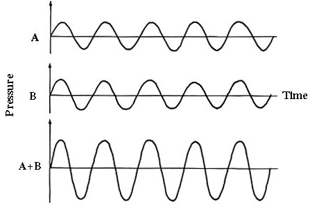
The linear superposition principle states that, at any given time, the total displacement of two superimposed vibrations (waves) is equal to the algebraic sum (i.e. a sum that takes into consideration signs: +, -) of the displacements of the original vibrations (waves).  First introduced by Bernoulli (late 1700s), this principle came out of the study of strings, considered as one-dimensional systems.  It stated that many sinusoidal vibrations can co-exist on a string independently of one another and that the total effect at any point is the algebraic sum of the individual motions. 
To be more precise, if the compound vibration at any point of a string is the algebraic sum of the individual vibrations, it is the sinusoidal waves (and not the vibrations) that can co-exist on a string independently of one-another.

The interference principle (see the animation, below) is an extension of the superposition principle. It states that, when two or more vibrations (waves) interact, their combined amplitude may be larger (constructive interference) or smaller (destructive interference) than the amplitude of the individual vibrations (waves), depending on their phase relationship.  When combining two or more vibrations (waves) with different frequencies (f1, A1 & f2, A2), their periodically changing phase relationship results in periodic alterations between constructive and destructive interference, giving rise to the phenomenon of Amplitude fluctuation: amplitude that fluctuates periodically over time between A1+A2 and A1-A2, at a rate equal to the frequency difference of the original vibrations (waves) |f1-f2|.

 

In the graphs, below, two sines A & B have the same amplitude A and the same starting phase, but different frequencies (f1 & f2). Adding them together will produce a complex signal (A+B) whose amplitude fluctuates between a max (2AA) and a min (0) value because their periodically changing phase relationship (gradually moving from perfectly in-phase to perfectly out-of-phase) results in a periodic and gradual move between constructive and destructive interference at a rate equal to |f1-f2|. Depending on their rate, such fluctuations can be perceived as beating (sound with slowly fluctuating level), roughness (rattling sound), or combination tones (tones additional to the original tones), to be described later in the semester.

(interactive tool exploring interference between two sines with different frequencies)

 

As an extreme example of destructive interference, if two vibrations (waves) have the same frequency, amplitude, and source location but a 1800 phase difference, the two vibrations (waves) will cancel one another, resulting in no vibration (wave) at all. Complete (or almost complete) destructive interference is often used in active noise and feedback reduction systems. According to a short story in the December 10, 2004 issue of New York Times, two 2005 Honda car models were the first to carry active noise reduction systems, based on this principle. Versions of this feature are by now commonplace in car manufacturing and, of course, headphones.
Sines A & B have the same frequency, amplitude, and phase (00 phase difference). Their addition results in total constructive interference: the combined signal's amplitude is equal to the algebraic sum of the initial amplitudes (assuming both signals originate from the same point in space).	Sines A & B have the same frequency and amplitude but a 1800 phase difference. Their addition results in total destructive interference: the combined signal has amplitude 0, which is, again, the algebraic sum of the two amplitudes. Since the sines are perfectly out of phase, at every moment in time their displacements have equal values but opposite signs, resulting in a sum of 0 (assuming both signals originate from the same point in space).

 

 

---

 

 

Physical attributes of acoustic waves - Part II

 

Sound waves - Inverse Square Law

 

Wave: Transfer of vibration energy across a medium (e.g. air, string, etc.). Waves originate in but are not equivalent to vibrations. Waves depend on the properties of the propagation-medium while vibrations do not. Sound waves in air are manifested as alternating condensations/compressions (pressure above atmospheric pressure) and rarefactions (pressure below atmospheric pressure) that spread away from the vibrating source longitudinally (i.e. parallel to the direction of vibration), in the form of pressure fluctuations. The video, below, is a visualization of sound waves caused by a vibrating string.

For signals of sound waves, the x axis represents either       a) time, outlining the wave's period         or     b) distance, outlining the wave's wavelength (i.e. the distance the wave will travel during a period). In case (a), the signal is temporal and describes how wave energy varies with time at a single point in space.        In temporal signals, the phase of a wave is different at different points in time, reflecting the vibration of air at a a given point in space. In case (b), the signal is spatial and describes how wave energy is spread in space at a given moment in time.        In spatial signals, the phase of a wave is different for adjacent points in space, because the vibration energy propagating through the air in the form of a wave reaches these points at different times. [Defining waves is a complex task. See this extended definition]   Simple/Sine Wave: Transfer of a simple harmonic motion across a medium. Complex Wave: Transfer of complex vibration/motion across a medium.

 

Wavelength (λ): The distance a wave travels during one vibration cycle.  Unit: meters/cycle. Wavelenght is a function of a vibration's period T (and,consequently, frequency f) and of the speed of wave propagation c within a given medium:   λ= c*T (equivalent to λ= c/f). For any given medium (air, water, wood, etc.), the higher the frequency the shorter the period and the shorter the wavelength.	(click here for a wavelength calculator)
Speed of sound (c): c = (E / ρ)0.5 where E is Young's modulus in N/m2 (measure of stiffness) and ρ is density in Kg/m3. For example: Speed of sound on a string with tension T and linear density ρ (density: mass per unit length): c = (T / ρ)0.5. Our key take-aways from this equation are:      the stiffer/tenser the medium (e.g. metal vs. wood vs. air; looser vs. tighter string or drumhead) the higher the speed of sound, while      the denser/more compact the medium (e.g. cold vs. hot air / water vs. wood) the lower the speed of sound.   See, below, for a visualization of the impact of stiffness on the speed with which sound waves propagate through a medium.      * In this animation, the distance among molecules per medium represents degree of bond strength (i.e. stiffness), not density.        As noted above, higher density corresponds to lower sound speed.
Speed of sound in air:    c = 345m/s at 210C     or    1130ft/s at 700F [C: temperature in Celsius - F: temperature in Fahrenheit]   The speed of sound increases with air temperature because higher temperature expands the air and reduces its density (if the air is unconstrained and free to expand), or increases its stiffness (if the air is constrained and cannot expand): cCelsius = 345 + (C-21)*0.6 m/s: The speed of sound increases by 0.6 m/s for each Celsius degree of increase in temperature. cFahrenheit = 1130 + (F-70)*1.1 ft/s: The speed of sound increases by 1.1 ft/s for each Fahrenheit degree of increase in temperature.
Unit conversions and formulas   1 foot = 0.3048 meters   1 meter = 3.281 feet C = (5/9)*(F-32)    F = (9/5)*C+32

 

Transverse waves: waves propagating perpendicularly to the motion of the vibration (e.g. waves on a string, waves on the front and back plates of a violin, waves on a drumhead, etc.)

 

Longitudinal waves: waves propagating parallel to the motion of the vibration (e.g. sound waves in air or other gases).
Images sources: https://waitbutwhy.com/2016/03/sound.html  -  https://www.acs.psu.edu/drussell/demos/waves/wavemotion.html
Source: Institute of Sound and Vibration Research

 

Inverse Square Law

Assuming that the energy from a vibrating source spreads away from the source in a spherical manner (this is the idealized case of a "point source," practically applicable only to low frequencies, with wavelengths much larger than the source's dimensions - see diffraction, next module), the Intensity of the resulting wave at a given point in space is inversely proportional to the square of the distance from the source. Since I = W/A and, for a sphere, A = 4πr2,  the intensity ratio at distances r1 and r2 from the center of the sphere will be I1 / I2 = (r2 / r1)2 [can you derive this from the equation I = W/A ?].  For example, doubling the distance from a source will reduce the Intensity by a factor of 2x2=4 and a loss of 6dB.

Increasing the distance tenfold will reduce the Intensity by a factor of 10x10=100 (20dB loss). Decreasing the distance by a factor of 100 will increase the Intensity by a factor of 100x100=10,000 (40dB gain). etc.

 

---

 

Standing Waves

 

Reminders:
The linear superposition principle states that, at any given time, the total displacement of two superimposed vibrations (waves) is equal to the algebraic sum (i.e. a sum that takes into consideration signs: +, -) of the displacements of the original vibrations (waves). 
The interference principle is an extension of the superposition principle. It states that, when two or more vibrations (waves) interact, their combined amplitude may be larger (constructive interference) or smaller (destructive interference) than the amplitude of the individual vibrations (waves), depending on their phase relationship. 

 

Standing waves are examples of the combination of constructive and destructive interference between a sound wave and its reflection(s). They are vibration patterns (on strings, air columns, listening environments, etc.) arising when energy propagating as a wave is trapped within two or more, appropriately positioned, reflective boundaries. Trapped waves create standing waves only if the distance between the boundaries is an integer multiple of the waves' half-wavelength. Consequently for a given distance d standing waves can be created at frequencies with wavelengths that are integer divisors of 2*d. Example: Assuming speed of sound c = 360m/s and two reflecting boundaries d = 6m apart. The longest-wavelength standing wave will be λ = 2d = 12m and will correspond to frequency f = c/λ = 360/12 = 30Hz Additional standing waves will be created with integer devisor wavelengths (12/2=6m; 12/3=4m; 12/4=3m; etc.) and, consequently, integer multiple frequencies (30x2=60Hz; 30x3=90Hz; 30x4=120Hz; etc.) Standing waves are characterized by fixed points along the wave propagation medium where the amplitude is maximum (antinodes) & minimum (nodes - nodes have a zero amplitude at the extreme case of no energy absorption at the reflective boundaries). They are a form of resonance and occur at an oscillating system's natural frequencies (see "Resonance" in the next module). Standing waves are desirable in musical instruments and undesirable in listening environments.   Transverse Standing Waves Transverse standing waves are quite common in string and percussion musical instruments. For example, transverse standing waves on a violin's stings and back plate are responsible for the majority of sonic energy generated by the instrument (which of the two, in your opinion, contributes most of the energy?). Transverse standing waves are also generated on drum skins, xylophone/vibraphone bars, and other solids used in musical instrument construction. The animation, to the right, illustrates complex patterns of transverse standing waves (referred to as Chladni patterns/figures) forming on a metal plate that is being excited at two different frequencies. Sand granules settle at the nodes. The animations below-right, simulate standing waves on a string. All these waves occur simultaneously, combining into a single signal (more under "spectrum" and during the following modules). (source) Longitudinal Standing Waves Longitudinal standing waves are generated inside any air cavity. Standing waves within the air cavities of musical instruments are useful and, in some cases necessary, amplifying and "coloring" the sound produced. Standing waves in air cavities outside a musical instrument (e.g. any enclosed listening space) are undesirable because they contribute to widely uneven sound level and frequency distribution within the space. (source) Interactive tool exploring standing waves (The Physics Classroom)

   

Interference of sound waves from sources separated by some distance A phenomenon analogous to standing waves on strings or air columns is observed if the two identical waves originate from two sources that are separated by some distance. The result is analogous to standing waves, but with an interference pattern (gradual shifts between constructive and destructive interference) spreading away from the sources and outlining areas of minimum (nodes) and maximum (antinodes) sound levels in space - a form of "moving" standing wave! In the following example, the animation portions with contrasting alternating colors correspond to areas of higher levels (maximum level at their center) and animation portions with minimal change in color correspond to areas of lower levels (minimum level at their center). This phenomenon arises, for example, whenever two or more loudspeakers produce exactly the same sound waves, as is the case during mono playback over a stereo system, or during many live sound reinforcement contexts that don't involve professional engineers.

Interference patterns and associated SPL (sound pressure level) spatial non-uniformity is particularly pronounced in open-air performances, where there are no reflections to diffuse wave energy and, potentially, improve SPL uniformity.

Play around with the interactive animation, below, to explore the relationship among sound source distance, sound wave frequency, and resulting interference patterns.

[source]

_ For a slightly different visualization, click here. _ For an interactive java applet with sound, click here.

 

---

 

Spectrum / Spectral Envelope - Fourier Analysis - Modulation

 

J. Fourier's (1768-1830) mathematical law states that all complex signals can be reduced to the sum of a set of sines. These are called the Fourier/sine components or partials of a complex signal and make up the complex signal’s spectrum.  Analysis of a complex signal into its sine components is called Fourier analysis. The reverse process of constructing a complex signal out of a set of sinusoids, is called Fourier synthesis. The equation, to the right, is a mathematical expression of this statement (we will not be performing any operations with this equation).  For periodic signals, also called harmonic signals (such as the signals corresponding to most musical sounds), the lowest frequency component is the 1st harmonic component or "the fundamental" (sometimes designated as ƒ0). All other harmonic components (also called harmonics) have frequencies that are integer multiples of the frequency of the fundamental. That is, if the fundamental component has frequency 1ƒ0, then the components above the fundamental have frequencies 2ƒ0, 3ƒ0, 4ƒ0 (referred to as 2nd, 3rd, 4th harmonic) and so forth.  All other types of signals are non-periodic and are called inharmonic.  The term "overtones" is occasionally also used to refer to any components with frequencies above that of the lowest component. They are designated as harmonic overtones to refer to to the upper components/harmonics of harmonic signals or inharmonic overtones to refer to the upper components of inharmonic signals. Periodic (harmonic) complex signals have a rather definite pitch that matches in frequency the frequency of the fundamental component. This appears to be the case even if the fundamental component is not present in the signal’s spectrum (more during the module on "pitch").
Non-periodic (inharmonic) signals have a rather indefinite pitch or no pitch at all, depending on the degree of inharmonicity (i.e. on how far away its frequency components are from an integer multiple relationship) and on the absolute and relative duration of their spectral components. More during the discussions on pitch, loudness, and timbre in the following weeks.
Experiment with this Fourier synthesis java applet.
Here is an additional Fourier Synthesis Simulation (save the file and open it with the Java console, available for download here). You may also download the Fourier-based Synthesizer used in class (Custom application, Windows only. To install, save the  SynthSetup.zip zipped file, double-click on it to un-package it, and run the SETUP.EXE file).

 

Spectrum   A two-dimensional graphic representation indicating the frequency (x axis) and amplitude/level//pressure/power (y axis) values of a signal's sinusoidal components. It is a "recipe," indicating the type (frequency) and amount (amplitude) of each ingredient (sine component) required to make the corresponding complex signal. Analogously to Signal Envelope, described in Part I of this module, the Spectral Envelope is a boundary curve that traces the peaks of the spectrum, capturing how energy is distributed across the frequency range (in the image: spectral components are in blue, spectral envelope is in black).
	Spectra always illustrate a signal's "recipe" for a specific time-slice, with multiple successive such time-slices illustrating how the signal's frequency energy distribution changes with time. For all musical signals, spectral distribution does change with time. Consequently, the amplitude (and secondarily the frequency) values of each spectral component also change with time. Differences in amplitude envelopes among a spectrum's sinusoidal components correspond to sound quality changes that we will discuss during the "Timbre" module. The "waterfall" visualization (left) is a 3-D spectrum that includes frequency (x axis), amplitude (z axis) and time (y axis). Spectral envelopes per time slice are displayed along the x (frequency) axis and amplitude envelopes per frequency component are displayed along the y (time) axis.    See and hear spectrograms of sample instruments.

 

	Graphical  example of synthesis: Complex signal made out of two sine components with frequencies f1 = 250Hz and f2 = 500Hz. The pitch of a complex tone corresponding to this complex signal would match the pitch of the fundamental component (250Hz). The graph below-left is the complex signal resulting from the addition of the two sine signals in the graph to the left. The graph below-right is the spectrum of the complex signal, indicating the frequency and amplitude values of the sine components making up the complex signal.
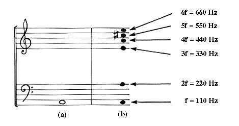
Relationship between harmonic frequency components and musical notation
Animation of the first 31 spectral components of a harmonic signal beginning at 110Hz, (tone with pitch A2), played back in sequence  (by Mladen Milicevic)	(a): A2 musical pitch (fundamental frequency: 110Hz), represented in musical notation. (b): the frequencies and (approximate) notational representation of the first six components of the tone in (a) (after Campbell and Greated (1987). Musician's Guide to Acoustics).

Ideal signal-forms and spectra, (also called 'waveforms')  Key: A: amplitude of the first component;  n: component number
(a) An ideal sawtooth signal (far right) is formed by summing an infinite number of harmonic components, with amplitudes A/n and 1800 phase-shift between odd- and even-numbered components, illustrated on the spectrum (right).   The blue points marking the amplitudes of the even components are on the opposite side of the blue points marking the amplitude of the odd components, to illustrate the phase shift.
(b) An ideal triangular signal (far right) is formed by summing an infinite number of only odd-numbered harmonic components, with amplitudes A/n2 and 1800 phase-shift between successive odd components, illustrated on the spectrum (right).
(c) An ideal square signal (far right) is formed by summing an infinite number of only odd-numbered harmonic components, in phase with one another and with amplitudes A/n, illustrated on the spectrum (right).

 

Animated spectra; 4 ideal signal-forms	(Different animation angle)
First 6 harmonic components of a sawtooth signal analogous to those generated by strings	Pitch/note values of each component of the signal to the left (assuming fundamental = 256Hz) & corresponding standing waves on a string
Experiment, again, with this Fourier synthesis java applet    [Optional: detailed discussion of spectra]

Fourier analysis drawbacks
Spectra arising from Fourier analysis are, unfortunately, never as clean and precise as the ones in the above figures.  The frequency values returned from the analysis are frequency ranges/bands, not precise frequency values (compare the spectral lines (left) vs. bands (right), below). There actually is a time/frequency trade-off in that: a) the more precisely we want to know how the energy of a spectrum changes with time, the less precisely the frequency values will be represented and b) the more precisely we want to know the frequencies in a spectrum, the longer the signal chunks analyzed will have to be and the less precisely the level changes of a sound over time will be captured.  In other words, we can only increase the frequency resolution of the analysis at the expense of the time resolution and the converse. This trade-off is related to Heisenberg's uncertainty principle, which states that the more precisely we determine the position of a particle the less precisely we may know its momentum (momentum = mass*velocity) and the converse. In addition, there is a series of assumptions accompanying the standard mathematical implementation of Fourier analysis: (a) the signal analyzed has infinite duration and (b) all the energy within a frequency band lays at the band's upper end. Violation of these assumptions results in spectral "smearing" (i.e. spectral components that are artifacts of the analysis process, surrounding the actual spectral components belonging to the signal - see below).
Frequency and amplitude values of the spectral components used to synthesize the complex signal to the right.	Complex signal synthesized by adding the two sinusoidal signals described by the spectrum to the left.	Spectrum resulting from Fourier analysis of 17ms-long portions of the same signal. Temporal resolution: 0.017s or 17ms  Frequency bandwidth: 1/0.017 =~ 59Hz.

 

Amplitude and Frequency Modulation
In broadcast technology, the terms Amplitude Modulation (AM) and Frequency Modulation (FM) describe two specific signal processing techniques used in the wireless transmission of audio signals. In simple terms, audio signals can be transmitted over large distances more robustly and with less contamination if they are "carried" by higher frequency signals, which a) have more energy (energy is proportional to the square of frequency), and b) can be transmitted/received by smaller antennas than those required for lower frequencies (the higher the frequency the shorter the wavelength). So, rather than being transmitted directly, the intended signal is transmitted in the form of a modulation (i.e. modification) of a high-frequency carrier signal. Most common application: AM and FM Radio.	High-frequency carrier (not shown) modified by a low-frequency signal (black) through amplitude modulation (producing the signal in red) or through frequency modulation (producing the signal in blue).
In its simplest case:   i) Sinusoidal Amplitude Modulation refers to the sinusoidal variation of a carrier signal's amplitude, at a rate equal to the modulating signal's frequency and at a degree (or depth) equal to the modulating signal's amplitude. The analogous musical term is "Tremolo," describing the sensation of slow loudness fluctuations, similar to the sensation associated with interference and "beating."   ii) Sinusoidal Frequency Modulation refers to the sinusoidal variation of a carrier signal's frequency, at a rate equal to the modulating signal's frequency and degree equal to twice / four times / six times, etc. the modulating signal's frequency, depending on "modulation index." The analogous musical term is "Vibrato," describing the sensation of slow pitch fluctuations.    In (a), below, the bottom signal is an AM signal, resulting when the top sine signal modulates the amplitude of a high-frequency carrier sine signal (not shown). In (b), a low-frequency sine (black) is modulating a high-frequency carrier sine (blue), resulting in the FM signal at the bottom (red).
(a)	(b)
Experiment with these AM & FM applets

 

Signal and spectral representations of amplitude-modulation rate and depth
Based on the above graphs, can you deduce the spectral correlates of the rate and depth parameters of amplitude modulation? (answer just below) Sinusoidal amplitude modulation [with modulation rate fmod (in Hz)  and modulation depth m (in %)] of a sine signal (with frequency f and amplitude A) results in a signal with a) amplitude that fluctuates above/below A by an amount that depends on the modulation depth and at a rate equal to the modulation rate, and   b) spectrum that has three components; the original sine (f; A) and two sidebands, also determined by the modulation rate and depth:     _ a low-frequency sideband,   flow  = f - fmod    -    Alow  = 1/2mA       _ a high- frequency sideband, fhigh = f + fmod   -    Ahigh = 1/2mA   (Ahigh = Alow)   In other words, modulation depth defines the energy shared by the two sidebands as a percentage of the energy of the original sine For example: If the amplitude of a sine signal (f = 2000Hz and A = 4) is modulated at a rate fmod = 10Hz and depth m = 60%  then        a) the resulting AM signal will have the same frequency (fAM = 2000Hz) but amplitude that fluctuates above/below A=4          at a rate equal to 10 times/second.      b) the spectrum of the resulting AM signal will have three components: the original sine (f = 2000Hz and A = 4) and two sidebands:      flow  = f - fmod  = 2000-10  = 1990Hz    -    Alow  = 1/2mA = 0.5*0.6*4 = 1.2      fhigh = f + fmod = 2000+10 = 2010Hz    -    Ahigh  = 1/2mA = 0.5*0.6*4 = 1.2

Loyola Marymount University - School of Film & Television