Basilar Membrane

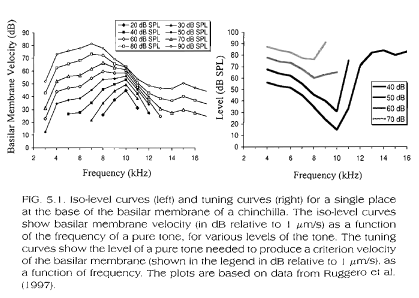
The filter shape of the basilar membrane (BM) response to pure tone stimuli changes with stimulus level.

More specifically, for high-frequency response positions on the BM (i.e. basal portions of the BM ~10KHz, see Fig. 5.1, below, for chinchilla data), as the stimulus intensity increases, the filter's bandwidth increases and the best frequency for a given BM location decreases.  So, as the level of sinusoidal stimuli exciting the basal portions of the BM increases, the perceptual results are:

• A larger area on the BM is stimulated, corresponding to a stimulation of a larger number of inner hair cells and, consequently to a distorted perception (one that includes not only the original sinusoid but additional ones, which correspond to the characteristic frequencies of all inner hair cells stimulated).

• The decrease in the 'best' frequency of a given place on the BM means that this place will respond best to a frequency lower than the characteristic frequency of the inner hair cells aligned with it. So, a strong sinusoid of a given frequency will end up exciting best an inner hair cell of a higher characteristic frequency, sending a higher frequency, and therefore pitch message to the brain than the pitch that would usually correspond to the sinusoid's actual frequency.

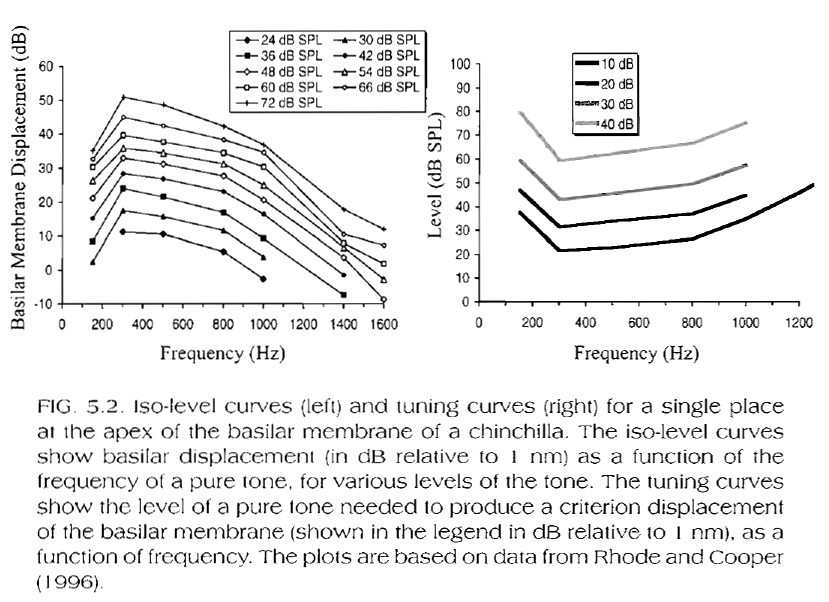
For lower-frequency response positions on the BM (i.e. apical portions of the BM ~500Hz, see Fig. 5.2, below, for chinchilla data), the filter's bandwidth and 'best' frequency do not change significantly with stimulus level increases.

It is practically very difficult (if not impossible) to obtain in-vivo (i.e. live) physiological measurements from even more apical locations (i.e. locations responding to frequencies lower than 500Hz) on the BM.  Perceptual experiments, however, indicate that, as the stimulus level increases, the perceived pitch of a low frequency tone decreases significantly.  This suggest that, in terms of 'best' frequency response, apical portions of the BM may respond in an opposite manner to basal portions (where, as the stimulus level increases, the perceived pitch of a high frequency tone also increases).

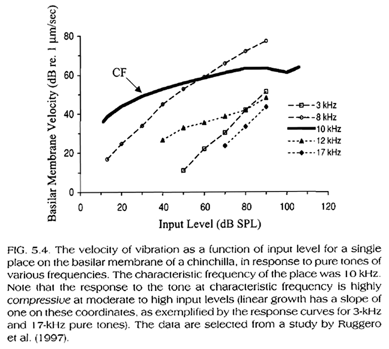
From the data in the above figures and in Fig. 5.4, below (presenting portions of the data in Fig. 5.1), we can draw an important conclusion:
The mechanical response of the BM is compressive at (and near) the best frequency of a given BM location (defined as the frequency at which a given BM portion responds best for low-to-moderate stimulation intensity levels), while it is linear at frequencies below or above this frequency.  More specifically, the mechanical response of the BM at (and near) the best frequency of a given BM location is more sensitive to low stimuli levels at this frequency than at other frequencies.  The response increases linearly for up to low-to-moderate stimuli levels, and compressively for higher stimulus levels.

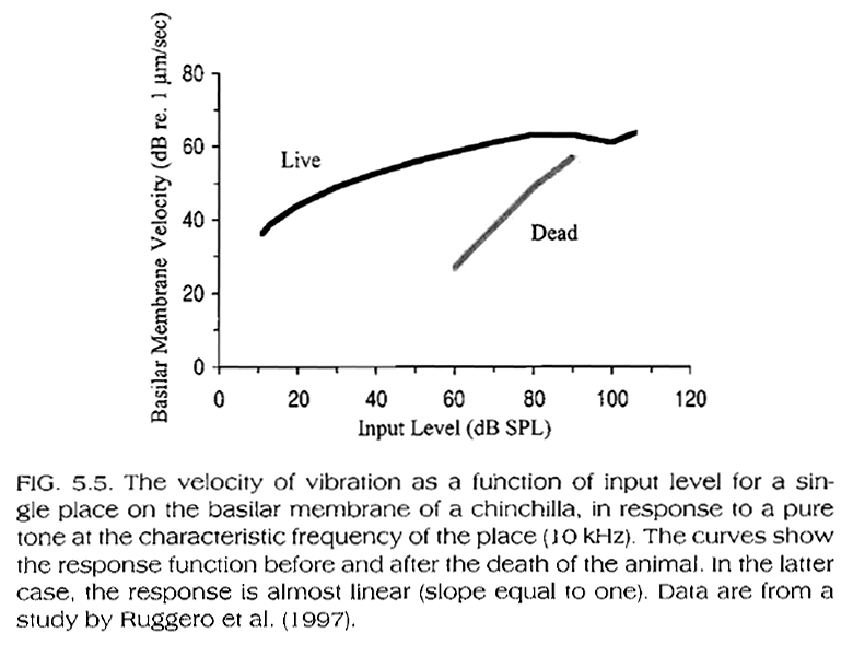
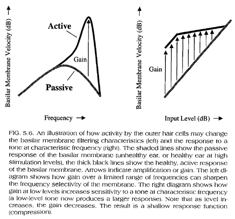
Based on Fig. 5.5, below (BM response of a live vs. a dead cochlea), we can also conclude that this compressive, nonlinear response of the BM is not due to its mechanical properties alone but to mechanical influences on the BM within a live cochlea.  As we have seen in Module 3a (see also Fig. 5.6, below), the compressive BM response in a live ear is due to the action of the outer hair cells, which, for a given 'best' frequency on the BM, amplify low-level stimuli (~10-40dB) more that they do high level stimuli (~40-80dB), while they actually help de-amplify or attenuate stimuli at very high levels (~80-110dB). At even higher levels, the outer hair-cell function is compromised.

 

 

             Auditory Nerve Fibers

The tuning curves of afferent auditory nerve fibers (i.e. nerve fibers connected to inner hair cells and taking messages from the ear into the brain) are expected to correspond to tuning curves obtained from a specific location on the BM, because each afferent nerve fiber innervates a single inner hair cell, which in turn is aligned with a single location on the BM.  The nerve fiber tuning curves in Fig. 5.7, below, are therefore very similar in shape to the BM tuning curves in fig. 5.1, above. 

One important point to note is that, although the filter bandwidths implied by these tuning curves seem to increase with characteristic frequency (e.g. the bandwidth in Hz increases with center frequency in the figure to the left, where the frequency axis is on a linear scale), the actual sharpness or Q factor of the filters (defined as the ratio of the filter's center frequency over the filter's bandwidth in Hz) increases and therefore the filter's effective bandwidth decreases (e.g. the bandwidth decreases with center frequency in the figure to the right, where the frequency axis is on a log scale).  In other words, although the auditory filter's bandwidth in Hz increases with increasing center frequency, the bandwidth relative the center frequency decreases.

Representing the auditory filter's bandwidth as a ratio rather than in absolute Hz values is consistent with
Weber's (Fraction) Law (1800s): The smallest detectable amount of change (ΔS) in a stimulus (S) is proportional to the
absolute (or "pedestal") magnitude of the stimulus.
So, ΔS/S = constant.  ΔS is also referred to as the Just Noticeable Difference or JND.
For example, for frequencies around 1000Hz, Δf/f ~ 0.002 and the JND for frequency for, say 800Hz is 800Hz * 0.002 = 1.6Hz (i.e. the frequency of a sinusoid at 800Hz must be raised to at least 801.6Hz if this change is to be perceptually noticed).

Auditory Nerve Fiber Distribution and Activity

• ~30,000 auditory nerve fibers linked to auditory hair cells
• ~ 90% of the nerve fibers are linked to the inner hair cells:
• A single inner hair cell may be connected to up-to 20 nerve fibers while up to 10 outer hair cells are connected to each nerve fiber.

• Spontaneous activity: Firing activity of a single neuron (nerve fiber) in the absence of a stimulus.  The discharge rate (i.e. number of electrical discharges per unit time) of spontaneous activity ranges from 0 to 100 spikes per second.

• Maximum activity. The theoretical maximum discharge rate of a neuron is ~ 1000 spikes/sec, although most auditory nerve fibers measured have discharge rates that max at ~ 500 spikes/sec.

• Single neuron threshold: The minimum stimulus level that will cause an increase in firing rate above the spontaneous discharge rate.

Neurons with low spontaneous discharge rate (SR-L) are less sensitive to stimulation and respond best to higher level stimuli. Since the response growth rate of the auditory system at higher input levels is compressive, the discharge rate of SR-L neurons increases slowly and saturates at high input levels. Neurons with high spontaneous discharge rate (SR-H) are more sensitive to stimulation and respond best to low level stimuli. Since the response growth rate of the auditory system at low input levels is amplified, the discharge rate of SR-H neurons increases quickly and saturates at low input levels.   It is clear that the auditory system needs neurons that cover the range of spontaneous discharge rates, to cover a large dynamic range of response and to best match the response characteristics of the basilar membrane. The figure to the right illustrates the different responses of neurons with low, medium, and high spontaneous discharge rates (the different spontaneous discharge rates are represented by the dotted lines).

As an additional example, Fig. 5.8, below, shows the firing rate of a low spontaneous rate neuron as a function of stimulus level. Compare this figure to Fig. 5.4, above.  Both, the basilar membrane and single neuron responses are more sensitive and compressive at characteristic rather than lower frequencies (i.e. they are less sensitive and steeper at frequencies lower than the characteristic frequency).

Suppression in the Auditory Nerve

When a second tone falls within the tuning curve of an already stimulated fiber, then the firing rate increases.  However, when it falls within the shaded regions in Fig. 5.9, below, the firing rate of the neuron decreases (i.e. it gets suppressed).

 

 

 

Masking / Detailed Slides
(1 slide per page & 6 slides per page, displayed below).