Timbre and Signal/Spectral
Time-Variance
(signal envelope, spectral flux, etc.)
The average spectrum of a complex signal describes the amount of energy in each of the signal's
frequency components (partials) but does
not describe how the amount of energy in a signal or spectrum changes with time, a change that also influences timbre.
Signal time-variance can be represented through
the
signal envelope.
Spectral
time-variance (spectral flux) can be represented through
time-variant spectra,
spectrograms, or
individual component amplitude/frequency envelopes.
Signal Time-Variance
The significance of
signal envelope to timbre can be demonstrated by playing a sound
backwards. The sound signal changes with time, while its average
spectral distribution remains the same.
Example 1
- Example 2
-
Example 3.
(based on experiments by Houtsma et
al., 1987).
REMINDERS:
Attack: The portion of the envelope
tracing the development of a sound signal towards its maximum amplitude. It
represents how energy is built up in a vibrating system and, in music, can be manipulated
through instrument generator excitation methods (bowing, plucking, striking with
a hard or soft mallet, etc.).
In signal synthesis
contexts, the short time between the attack and steady
state portions
of a signal, during which the source generator's response
settles following initial excitation, is referred to as "decay."
Prior to the advent of
synthesizers, the term "decay" had been used to describe the
final signal
portion, now referred to as "release." In the
context of acoustics, decay is a more appropriate term
for the last portion of a signal envelope.
Steady state: The
portion of the envelope corresponding to a vibrating system's
response to the continuous supply of energy, modulated via performance techniques such as vibrato, muting, damping,
bowing pressure, driver excitation location, etc..
Decay (Release):
The portion of the envelope that traces the drop in amplitude
(or "decay") of a sound signal from its maximum value to zero,
following the "release" of the source's generator from excitation.
Decay occurs when energy stops being supplied to a vibrating
system, and represents how energy stored in a system eventually
dissipates.
Decay time depends on:
-
The resonance and feedback characteristics of the vibrating system.
More specifically, the sharper a resonator's tuning and the
less the feedback in the vibrating system the shorter the
decay time.
-
The environment
within which the
system vibrates. More specifically, the less boundaries
around the vibrating system and the lower their
reflectivity, the shorter the decay time.


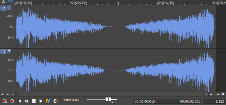
Based on envelope shapes, we classify signals in two broad categories:
i)
Continuous signals (image above, left),
where most of the energy is contained in the steady state
portion of the
envelope (e.g. signal of a bowed violin string).
ii)
Impulse signals (image above right),
where the envelope has no steady state portion and the attack portion is much shorter and steeper than
the
decay portion (e.g. signal of a struck, marimba bar).
The attack portion of the signal envelope
contains a signal's onset transients:
frequency components that are
a) usually inharmonic,
b) reach higher amplitudes than other components,
c) die
out rather fast, and
d) contribute to a signal's
perceived
degree of
noisiness/naturalness.
The attack influences the timbre of any
signal
but significantly more so that of impulse signals. In this
example,
three orchestral instruments are presented with the
attack portion of their signal removed. Can you recognize the
instruments? If yes, which instrument's sound has been impacted more
by the removal of the attack? [ key at the bottom of the page ].
NOTE: The separation between a signal envelope's sections
is, in most cases, not clear-cut
(especially between attack and steady state).
In
addition, the so-called "steady state" represents a portion
of the signal during which several of its acoustical
parameters are changing.
Spectral Time-Variance
Spectral
time-variance describes changes in the frequency and amplitude of a
complex tone's components with time. It can be represented by:
A) Time-variant
spectra: 3D "waterfall" plots; usually with frequency on the x axis, time on the y
axis, and level on the z axis.


Click here
for a video of the time-variant spectrum of all 3 piano examples,
mentioned above (Houtsma et al., 1987).
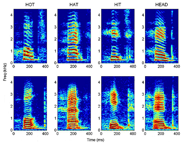
B) Spectrograms:
2D plots; usually with time on the x axis, frequency on the y
axis, and intensity in different color shades.
See and hear 2D Spectrograms of sample sound sources.


Spectrograms from (a) warbler, (b) whale, (c) flute, (d) singer singing a steady tone.
(from "Music without Borders"
by Susan Milius) |
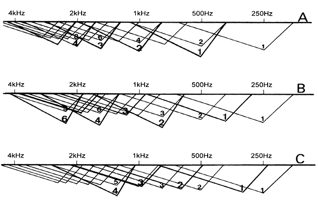
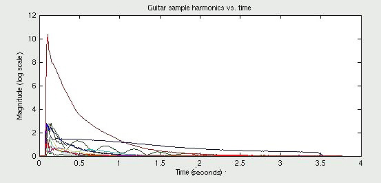
C) Amplitude
(or, less
commonly, frequency) envelopes of the individual spectral components: 2D plots, usually with time on the x axis, level
(or frequency) change on the y
axis, and spectral component frequency or number in different color/style
lines:
Spectral time-variance contributes to the
"naturalness" of a sound, while deviations from harmonic spectra and the way these interact when
several instruments perform together in unison change the timbre of the
resulting sound and contribute to its 'liveliness' and what is perceived as a 'chorus effect'.
|
Timbre, Duration, & Time Separation
As discussed previously, there is
a
-
duration threshold for
loudness (~200ms for sine signals; ~400ms for broadband signals),
below which loudness appears to increase with increase in duration, even if
the sound intensity level remains fixed, and
-
duration
threshold for pitch (~10-60ms, depending on frequency and intensity)
below which sounds lose their pitch identity.
Durations that are shorter than a given signal's
attack portion significantly degrade timbre perception.
In addition, two signals separated by a time delay
that is shorter than a specific time separation threshold of ~2-50ms,
depending on the spectra of the two signals, sound
as one (per Hirsch, 1959; details and analysis in
Divenyi, 2004). In
this case, introduction of the second, delayed signal has an effect on the
original signal's:
-
loudness (the loudness of the original signal appears to
increase) and
-
timbre (the original signal's attack portion becomes less sharply defined, resulting in a timbre with
a rather 'blurry' onset).
This
example
presents 3 complex signals with fundamental 600Hz.: (i) a single complex tone, (ii) two complex tones
separated by 30ms, and (iii) two complex
tones separated by 150ms. The
introduction of the second tone in (ii) is perceived as an increase in
loudness and a change in the attack of the first tone. The
introduction of the second tone in (iii) results in the perception of two
tones with two distinct onsets.
Duration and time separation thresholds
are linked to the mechanical and electro-chemical latency of the
auditory system and the associated forward masking effect.
Previous experience and context can override such psycho-physiological
limits, allowing listeners to make pitch, loudness, and timbre judgments for tones
with durations below the suggested thresholds.
Listen to a melody performed using 7 notes shortened to clicks (2 signal
cycles per note).
Stripped from context, this melody is unrecognizable, to most listeners. If listeners are told
that this is the opening line of "......(look at the bottom of the
page)..." they are able to
hear the intended pitch contour. After listeners have been primed to
listen to this tune, some may continue to hear it
even if the "notes" represented by each click
follow a random pitch pattern.
|